
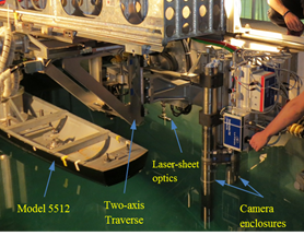
Model 5512 mounted to the PMM carriage with the towed, TPIV system in the foreground supported by the PMM carriage strongback. The underwater camera enclosures and laser-sheet generator (all submerged) are visible in the image.
Experiment
Towing tank experiments were performed for a surface combatant for static drift maneuvers with different drift angles. Measurements include global force and moment, wave elevations, and local mean-flow fields. The geometry is model 5512, a 3.048 m geosim of DTMB model 5415. The experiments were performed in a 3 m ´ 3 m ´ 100 m towing tank at the Iowa Institute of Hydraulic Research (IIHR), University of Iowa. The measurement system features a planar motion mechanism (PMM), a towed underwater tomographic particle image velocimetry (TPIV) system, servo-type wave gauges, and a 6-component loadcell. The quality of the data was assessed by monitoring statistical convergence and following standard uncertainty analysis procedures. The mean vortical flow structures of the volumetric measurement data were cross-referenced with computational simulations for identification of the flow vortices around the hull. An onset, separation and progression analysis was performed for the major vortices identified. For a better understanding of the complex flow, the analysis of the measured flow is presented together with the computational study by Bhushan et al. (2014).
Data, Equipment, and Conditions
| Data | Equipment | Fr | Drift angle, b (°) |
| Local flow field | TPIV | 0.28 | 0, 10, 20 |
| Global forces and moment | Load cell | 0.28 | 0, ±2, ±6, ±9, ±10, ±11, ±12, ±16, ±20 |
| Free surface elevation | Servo type wave gauges | 0.28 | 0, 10, 20 |
Sample Images
The following photo shows model 5512 mounted to the PMM carriage with the towed, TPIV system in the foreground supported by the PMM carriage strongback. The underwater camera enclosures and laser-sheet generator (all submerged) are visible in the image.
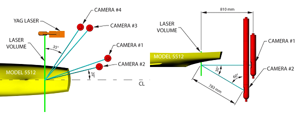
The following images show the top (left) and side (right) views of the TPIV layout in the horizontal and vertical planes, respectively.
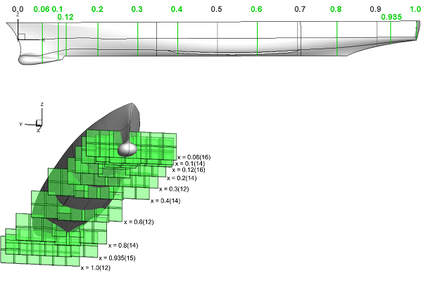
The following images show the TPIV measurement stations (top; the green lines) and the measurement volume allocations (bottom; the green boxes) at each station for the b = 10° case. The numbers in the parenthesis are the total number of TPIV volumes at each station.
Sample Data
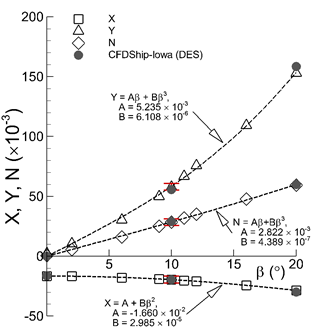
The following image shows experimental surge X and sway Y forces and yaw moment N coefficients at various drift angles and comparisons with the CFDShip-Iowa simulations. The red error bars represent the uncertainty limits of the experimental data.
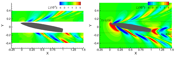
The following images show wave contours at b = 10° by the present experiment (left) and the CFDShip-Iowa simulation (right).
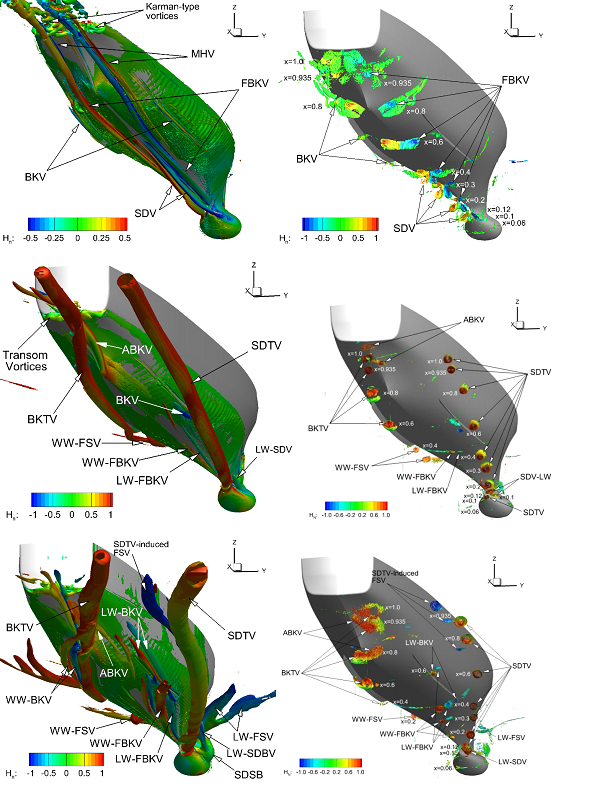
The following figures show the iso-Q surfaces colored by the normalized helicity level Hn for b = 0° (top), 10° (middle) and 20° (bottom) by CFDShip-Iowa anisotropic DES on 84M grid (left) and TPIV (right).
References:
Bhushan, S., Yoon, H., Stern., F., Guilmiuau, E., Visonneau, M., Toxopeus, S., Simonsen, C., Aram, S., Kim, S-E, Griporopoulos, G., Petterson, K., and Fureby, C., 2015, “CFD Validation for Surface Combatant 5415 Straight Ahead and Static Drift 20 Degree Conditions,” IIHR—Hydroscience & Engineering, The University of Iowa, IIHR Technical Report #493.
Bhushan, S., Yoon, H., and Stern, F., 2016, “Large grid simulations of surface combatant flow at straight-ahead and static drift conditions,” International Journal of Computational Fluid Dynamics, Vol. 30, No. 5, pp. 356-362.
Bhushan, S., H., Yoon, F., Stern, E., Guilmineau, M., Visonneau, S., Toxopeus, C., Simonsen, S., Aram, S., Kim, and G., Grigopoulos, 2016, “Verification and Validation of CFD for Surface Combatant 5415 for Straight Ahead and 20 Degree Static Drift Conditions,” SNAME Transactions, Vol. 123, pp. 1-26.
Bhushan, S., Yoon, H., Stern, F., Visonneau, M., Guilmineau, E., Toxopeus, S., Simonsen, C., Aram, S., Kim, S-E., and Grigoropoulos, G., “Assessment of CFD for Surface Combatant 5415 at Straight Ahead and Static Drift,” Journal of Fluids Engineering (under review), 2017.
Yoon, H., Gui, L., Bhushan, S., and Stern, F., “Tomographic PIV Measurements For Surface Combatant 5415 Straight Ahead and Static Drift 10 and 20 Degree Conditions,” 30th Symposium on Naval Hydrodynamics, Hobart, Tasmania, Australia, 2014.